Where to open a Restaurant in LA County, CA?

Coursera Capstone Project

Finding a location and type for a restaurant in Los Angeles County, CA

Table of contents

• Introduction: Business Problem
• Data
• Methodology
• Analysis
• Results and Discussion
• Conclusion

Introduction: Business Problem

In this project I will try to give a recommendation on where to open a restaurant in Los Angeles County, CA. In addition, there shall be given a recommendation of which type of restaurant could be opened, based on existing restaurants in the area and generally popular restaurants in the whole county.

The decision on where to open a restaurant can be based on many factors, depending on the target group. For example, one could look for very dense populated areas, or areas with lots of wealthy citizens. Even the median age of the population can play a role.

I will make a decision based on the following conditions: - Find the area with a good balance between number of possible customers and a high median income (population is slightly more important than income) - the type of restaurant will be determined by the most recommended categories of food venue in Los Angeles County, CA and the number of already existing venues in the area

Data

I used three different datasets as basis for my analysis. Using these datasets I am able to work with the following features, among others: - A list of areas in Los Angeles County, CA based on the ZIP code - The number of citizens and households in every area - The estimated median income of every area - The latitude and longitude for every zip code in the county

I combined the following datasets for this: - 2010 Los Angeles Census Data - https://www.kaggle.com/cityofLA/los-angeles-census-data - Median Household Income by Zip Code in 2019 - http://www.laalmanac.com/employment/em12c.php - US Zip Code Latitude and Longitude - https://public.opendatasoft.com/explore/dataset/us-zip-code-latitude-and-longitude/information/

To analyse the existing food venues in the county, the Foursquare API is used. With this API we can provide the data to answer the following two questions: - What are the most recommended types of restaurants in the county? - What are the existing food venues categories in the area where we want to open a restaurant in?

Merging the three datasets as basis of the analytics

First, let’s merge all three datasets and get rid of unnecessary information. I will continue to use a single dataframe with the combined datasets as basis for further analysis.

The census data and the geodata for the US zip codes are available as csv files that I will read directly into a dataframe. The records for the median household income are available on a website, so I downloaded the data as a html file, which then is used to create a dataframe. As the median income has a dollar sign and can not be converted into a numeric value automatically because of its format, we have to do some data preparation.

import pandas as pd
from pathlib import Path
census_path = Path.cwd().joinpath('resources').joinpath('2010-census-populations-by-zip-code.csv')
html_path = Path.cwd().joinpath('resources').joinpath('Median Household Income By Zip Code in Los Angeles County, California.html')
zip_path = Path.cwd().joinpath('resources').joinpath('us-zip-code-latitude-and-longitude.csv')

# Dataset: 2010 Los Angeles Census Data
df_census = pd.read_csv(census_path)
# Dataset: Median Household Income by Zip Code in 2019
dfs = pd.read_html(html_path)
df_income_all = dfs[0]
# drop areas where the median income is missing
df_income_na = df_income_all[df_income_all['Estimated Median Income'].notna()]
# Next step: clean the values in the median income column to retrieve
# numeric values that can be used for clustering / calculation
df_income = df_income_na.drop(df_income_na[df_income_na[
                             'Estimated Median Income'] == '---'].index)
df_income['Estimated Median Income'] = \
    df_income['Estimated Median Income'].map(lambda x: x.lstrip('$'))
df_income['Estimated Median Income'] =\
    df_income['Estimated Median Income'].str.replace(',','')
df_income["Estimated Median Income"] =\
    pd.to_numeric(df_income["Estimated Median Income"])
# Dataset: US Zip Code Latitude and Longitude
df_geodata = pd.read_csv(zip_path, sep=';')
# Let's start by joining the geodata on the income dataset via the zip code
df_income_geo = df_census.join(df_income.set_index('Zip Code'), on='Zip Code')
# Now join the census data with the income dataset and the geodata
dataset_geo = df_income_geo.join(df_geodata.set_index('Zip'), on='Zip Code',
                           how='left')
# Let us only use the columns we need for the further analysis and ignore
# the rest
prepared_ds = dataset_geo[[
  "Zip Code", "City", "Community", "Estimated Median Income",
  "Longitude", "Latitude", "Total Population", "Median Age",
  "Total Males", "Total Females", "Total Households",
  "Average Household Size"]]
# last stop: let's drop records with missing data
final_ds = prepared_ds.dropna(axis=0)
final_ds.shape

(279, 12)

So the final dataframe now contains 279 areas with 12 features.
Let’s get an overview on how the records are looking:

final_ds.head(5)

	Zip Code	City	Community	Estimated Median Income	Longitude	Latitude	Total Population	Median Age	Total Males	Total Females	Total Households	Average Household Size
1	90001	Los Angeles	Los Angeles (South Los Angeles), Florence-Graham	43360.0	-118.24878	33.972914	57110	26.6	28468	28642	12971	4.40
2	90002	Los Angeles	Los Angeles (Southeast Los Angeles, Watts)	37285.0	-118.24845	33.948315	51223	25.5	24876	26347	11731	4.36
3	90003	Los Angeles	Los Angeles (South Los Angeles, Southeast Los ...	40598.0	-118.27600	33.962714	66266	26.3	32631	33635	15642	4.22
4	90004	Los Angeles	Los Angeles (Hancock Park, Rampart Village, Vi...	49675.0	-118.30755	34.077110	62180	34.8	31302	30878	22547	2.73
5	90005	Los Angeles	Los Angeles (Hancock Park, Koreatown, Wilshire...	38491.0	-118.30848	34.058911	37681	33.9	19299	18382	15044	2.50

Finding the most recommended food venue categories in the county

Now we will use the Foursquare API to find out what are the most recommended food venues in the county. For this we will go through every single area and get the recommended food venues in the vicinity of the area center.

# first, lets import the necessary libraries and the credentials for the API
from modules import foursquare
import requests
CLIENT_ID = foursquare.CLIENT_ID
CLIENT_SECRET = foursquare.CLIENT_SECRET
ACCESS_TOKEN = foursquare.ACCESS_TOKEN
VERSION = '20210514' # Foursquare API version
LIMIT = 100

# first, we use a list of the areas and without columns we don't need
areas = final_ds.drop(['Estimated Median Income', 'Total ' 'Population',
                        'Median Age', 'Total Males', 'Total Females',
                        'Total Households', 'Average Household Size'], 1)
areas.head()

FutureWarning:

In a future version of pandas all arguments of DataFrame.drop except for the argument 'labels' will be keyword-only

	Cluster Label	Zip Code	City	Community	Longitude	Latitude
1	2	90001	Los Angeles	Los Angeles (South Los Angeles), Florence-Graham	-118.24878	33.972914
2	2	90002	Los Angeles	Los Angeles (Southeast Los Angeles, Watts)	-118.24845	33.948315
3	2	90003	Los Angeles	Los Angeles (South Los Angeles, Southeast Los ...	-118.27600	33.962714
4	2	90004	Los Angeles	Los Angeles (Hancock Park, Rampart Village, Vi...	-118.30755	34.077110
5	2	90005	Los Angeles	Los Angeles (Hancock Park, Koreatown, Wilshire...	-118.30848	34.058911

In the next code block, we will iterate through every area in the dataframe and get up to 50 recommendations per area. For that I use the “explore” endpoint of the Foursquare API. I use the categoryId and sortByPopularity parameters to only request food venues that are sorted by popularity in descending order.

venues_list = []
for index, area in areas.iterrows():
    url = 'https://api.foursquare' \
      '.com/v2/venues/explore?&client_id={}&client_secret={}&v={}&ll={},' \
      '{}&radius={}&limit={}&offset={}&categoryId={}&sortByPopularity={}'\
        .format(
    CLIENT_ID, CLIENT_SECRET, VERSION, area['Latitude'], area['Longitude'],
    1000, LIMIT, 0, '4d4b7105d754a06374d81259', 1)

    results = requests.get(url).json()["response"]['groups'][0]['items']
    for v in results:
        try: # try to extract the city, if there is one in the response
            city = v['venue']['location']['city']
        except:
            city = area['City']

        try: # try to extract the zip code, if there is one
            postalCode = str(v['venue']['location']['postalCode'])
        except:
            postalCode = str(area['Zip Code'])
        # build a list with all the columns I want to use
        if postalCode == str(area['Zip Code']):
            venues_list.append((
                        area['Zip Code'],
                        area['Community'],
                        area['Latitude'],
                        area['Longitude'],
                        v['venue']['name'],
                        v['venue']['categories'][0]['name'],
                        city ))
# create a dataframe from the results of the request
la_venues = pd.DataFrame(venues_list, columns=['Zip Code', 'Community',
              'Zip Code Latitude', 'Zip Code Longitude', 'Venue',
              'Venue Category', 'City'])

la_venues.head()

	Zip Code	Community	Zip Code Latitude	Zip Code Longitude	Venue	Venue Category	City
0	90001	Los Angeles (South Los Angeles), Florence-Graham	33.972914	-118.24878	Mi Lindo Nayarit Mariscos	Mexican Restaurant	Los Angeles
1	90001	Los Angeles (South Los Angeles), Florence-Graham	33.972914	-118.24878	Jack in the Box	Fast Food Restaurant	Los Angeles
2	90001	Los Angeles (South Los Angeles), Florence-Graham	33.972914	-118.24878	Mi Lindo Nayarit	Seafood Restaurant	Los Angeles
3	90001	Los Angeles (South Los Angeles), Florence-Graham	33.972914	-118.24878	SUBWAY	Sandwich Place	Los Angeles
4	90001	Los Angeles (South Los Angeles), Florence-Graham	33.972914	-118.24878	El Senor Taco	Mexican Restaurant	Los Angeles

la_venues["Venue"].count()

8692

So we have found 8,692 recommendations for our 279 areas in Los Angeles County, CA. That are ~31 recommendations per area. Let’s extract the city and venue category and group the data by category, to find out about the distribution of the recommended food venue categories.

venues = la_venues[['City', 'Venue Category']]
categories = venues.groupby('Venue Category').size().to_frame('Count').reset_index()
sorted = categories.sort_values(by='Count', ascending=False) # Sort by Count
top10 = sorted.iloc[0:9] # Show the top 10 categories
top10

	Venue Category	Count
76	Mexican Restaurant	833
88	Pizza Place	575
40	Fast Food Restaurant	501
22	Chinese Restaurant	417
8	Bakery	347
98	Sandwich Place	342
1	American Restaurant	316
17	Café	304
13	Burger Joint	264

After that, we will visualize the distribution.

import plotly.express as px
from IPython.display import HTML, display
top15 = sorted.iloc[0:14]
fig = px.bar(top15, x="Venue Category", y="Count",
             title='Distribution of recommended food venue categories')
HTML(fig.to_html(include_plotlyjs='cdn'))
#fig.show(renderer='notebook_connected')

So with this data we can tell what food venue categories are recommended the most throughout Los Angeles County, CA.

We have prepared the following data, which we will use for further analysis: - a dataframe with areas in LA County, enriched with geodata, median income and census data - a dataframe with the most recommended food venue categories in the county

Methodology

In this project we will focus on finding a suitable area for a new restaurant in Los Angeles County, CA. The areas are defined by their US Zip Code. In addition, we will look at the most recommended food venue categories throughout the country, to suggest which type of restaurant could be opened. There won’t be a specific location in the chosen area recommended.

In the first step we have merged three different datasets, that provide data on the different areas in Los Angeles County. With this data it is possible to cluster the areas using information like median income, number of households and number of inhabitants. In addition, using Foursquare, we identified the most recommended food venue categories in the county.

The second step in the analysis is to cluster (using k-means clustering) the areas in the county and to describe the individual clusters. Using this method we support the process of finding a single area that looks promising for a new restaurant.

The third step is to pick a cluster that fits the chosen criteria most. The area shall be chosen under the premise of finding a good balance between estimated median income and number of potential customers. So the target is to find an area that has as many citizens as possible with the highest income possible. After an area was chosen, the distribution of local restaurant types in this area will be analysed. Combining this information with the categories of food venues that are popular throughout the county, a recommendation of the restaurant to open can be given.

Analysis

Getting an overview

First of all, let’s have a look on our dataset describing the areas.

final_ds.head()

	Zip Code	City	Community	Estimated Median Income	Longitude	Latitude	Total Population	Median Age	Total Males	Total Females	Total Households	Average Household Size
1	90001	Los Angeles	Los Angeles (South Los Angeles), Florence-Graham	43360.0	-118.24878	33.972914	57110	26.6	28468	28642	12971	4.40
2	90002	Los Angeles	Los Angeles (Southeast Los Angeles, Watts)	37285.0	-118.24845	33.948315	51223	25.5	24876	26347	11731	4.36
3	90003	Los Angeles	Los Angeles (South Los Angeles, Southeast Los ...	40598.0	-118.27600	33.962714	66266	26.3	32631	33635	15642	4.22
4	90004	Los Angeles	Los Angeles (Hancock Park, Rampart Village, Vi...	49675.0	-118.30755	34.077110	62180	34.8	31302	30878	22547	2.73
5	90005	Los Angeles	Los Angeles (Hancock Park, Koreatown, Wilshire...	38491.0	-118.30848	34.058911	37681	33.9	19299	18382	15044	2.50

Now we are going to take a look at the areas with the highest income and the highest population.

# sort descending by the income and draw the top 15 areas
income_sorted = final_ds.sort_values(by='Estimated Median Income',
                                     ascending=False)
income_top15 = income_sorted.iloc[0:14]
fig = px.bar(income_top15, x="Estimated Median Income", y="City",
 orientation = "h", color='Estimated Median Income',
             title='Distribution of Estimated Median Income')
HTML(fig.to_html(include_plotlyjs='cdn'))
#fig.show(renderer='notebook_connected')

# sort descending by the population and draw the top 15 areas
pop_sorted = final_ds.sort_values(by='Total Population',
                                     ascending=False)
pop_top15 = pop_sorted.iloc[0:14]
fig = px.bar(pop_top15, y="Total Population", x="City",
 orientation = "v", color='Total Population',
             title='Distribution of Population')
HTML(fig.to_html(include_plotlyjs='cdn'))
#fig.show(renderer='notebook_connected')

As we are primarily interested in the areas that have a high total population, let us add the income to this graph and get an overview on which areas in this group have the highest income.

fig = px.scatter(pop_top15, x="Estimated Median Income", y="Community",
                 size="Total Population", log_x=True, color="Total Population")
HTML(fig.to_html(include_plotlyjs='cdn'))
#fig.show(renderer='notebook_connected')

In this graph the population determines the bubble size. So there are four areas that stand out:

City	Population	Median Income
Norwalk	105,6K	70,7K
Lake View Terrace, Sylmar	91,7K	74K
La Puente, Valinda	85K	71,2K
Hansen Hills, Pacoima	104K	64K

These four cities / neighbourhoods seem to be suitable areas, based on their combination of population and median income. We are going to see, if this assumption is confirmed going forward.

Clustering the dataset

from sklearn.cluster import KMeans
grouped_clustering = final_ds.drop(['Zip Code', 'City', 'Community', 'Longitude', 'Latitude', 'Total Males',
                                    'Total Females'], 1)
grouped_clustering.head()

FutureWarning:

In a future version of pandas all arguments of DataFrame.drop except for the argument 'labels' will be keyword-only

	Estimated Median Income	Total Population	Median Age	Total Households	Average Household Size
1	43360.0	57110	26.6	12971	4.40
2	37285.0	51223	25.5	11731	4.36
3	40598.0	66266	26.3	15642	4.22
4	49675.0	62180	34.8	22547	2.73
5	38491.0	37681	33.9	15044	2.50

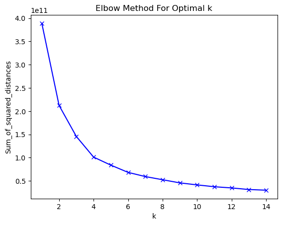
sum_of_squared_distances = []
K = range(1,15)
for k in K:
    kmeans = KMeans(n_clusters=k, init="k-means++",
                random_state=0).fit(grouped_clustering)
    sum_of_squared_distances.append(kmeans.inertia_)

#kmeans.labels_

C:\Users\schul\miniconda3\lib\site-packages\sklearn\cluster\_kmeans.py:881: UserWarning:

KMeans is known to have a memory leak on Windows with MKL, when there are less chunks than available threads. You can avoid it by setting the environment variable OMP_NUM_THREADS=2.

import matplotlib.pyplot as plt
plt.plot(K, sum_of_squared_distances, 'bx-')
plt.xlabel('k')
plt.ylabel('Sum_of_squared_distances')
plt.title('Elbow Method For Optimal k')
plt.show()

According to the elbow method I chose a k of 6 going forward. So let’s do the clustering again with the determined k value. Then I will add the cluster labels to my dataset and print out a summarization of the created clusters.

# cluster with the determined K
kmeans = KMeans(n_clusters=6, init="k-means++",
                random_state=0).fit(grouped_clustering)
# add the labels to the dataset
final_ds.insert(0, 'Cluster Label', kmeans.labels_)

# create a dataframe for the defined clusters
cluster_df = final_ds.groupby('Cluster Label').mean()
cluster_df

	Zip Code	Estimated Median Income	Longitude	Latitude	Total Population	Median Age	Total Males	Total Females	Total Households	Average Household Size
Cluster Label
0	90944.044444	51793.866667	-118.206034	34.081385	18356.955556	35.786667	9296.088889	9060.866667	6044.355556	2.850444
1	90624.000000	155063.444444	-118.425995	34.024770	17967.666667	43.838889	8777.833333	9189.833333	7020.722222	2.479444
2	90645.573770	52440.918033	-118.253427	34.038718	49920.491803	32.331148	24696.983607	25223.508197	15608.819672	3.248852
3	91028.756410	79091.974359	-118.215469	34.065151	29618.141026	38.174359	14394.820513	15223.320513	10698.910256	2.776026
4	90971.672727	105903.872727	-118.327527	34.099429	29382.745455	41.198182	14361.127273	15021.618182	11328.072727	2.540727
5	91153.090909	57912.863636	-118.190515	34.113848	83146.500000	30.468182	41257.500000	41889.000000	22069.545455	3.768182

Let us clean this up a bit and add a new column, that will help us to chose a cluster going forward.

clusters = cluster_df[['Estimated Median Income', 'Total Population',
                       'Median Age', 'Total Households', 'Average Household '
                                                         'Size']]

clusters['Decision Factor'] = \
    ( ( clusters['Total Population'] * 1.2 ) *
      clusters['Estimated Median Income']) / 100000
clusters_r = clusters.round(2)
clusters_r
clusters_sorted = clusters_r.sort_values(by='Decision Factor', ascending=False)
clusters_sorted

SettingWithCopyWarning:


A value is trying to be set on a copy of a slice from a DataFrame.
Try using .loc[row_indexer,col_indexer] = value instead

See the caveats in the documentation: https://pandas.pydata.org/pandas-docs/stable/user_guide/indexing.html#returning-a-view-versus-a-copy

	Estimated Median Income	Total Population	Median Age	Total Households	Average Household Size	Decision Factor
Cluster Label
5	57912.86	83146.50	30.47	22069.55	3.77	57783.02
4	105903.87	29382.75	41.20	11328.07	2.54	37340.96
1	155063.44	17967.67	43.84	7020.72	2.48	33433.54
2	52440.92	49920.49	32.33	15608.82	3.25	31414.52
3	79091.97	29618.14	38.17	10698.91	2.78	28110.69
0	51793.87	18356.96	35.79	6044.36	2.85	11409.33

Looking at these clusters, they can be described as the following:

Name	Income	Population	Age
Cluster 4	High	Medium	Older
Cluster 0	Low	Low	Young
Cluster 1	Very High	Low	Older
Cluster 5	Medium	Very High	Very Young
Cluster 2	Low	High	Very Young
Cluster 3	High	Medium	Young

So based on this information I am going to choose Cluster 5 for further evaluation and as the cluster where I will pick an area from. This cluster has a medium income combined with a very high population. It also contains the youngest median age, which also can be considered for choosing the food venue category.

cluster5 = final_ds.loc[final_ds['Cluster Label'] == 5, final_ds
    .columns[[1] + list(range(2, final_ds.shape[1]))]]
cluster5.shape

(22, 12)

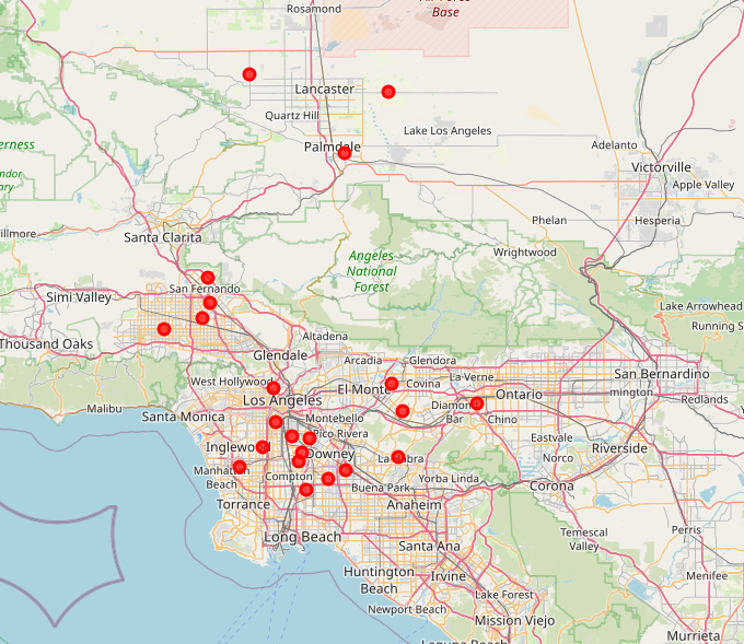
This cluster contains 22 areas in Los Angeles County, CA. We are going to have a look on them on the map using Folium.

from geopy.geocoders import Nominatim
# initialize the map
address = 'Los Angeles County, CA'
geolocator = Nominatim(user_agent="la_explorer")
location = geolocator.geocode(address)
latitude = location.latitude
longitude = location.longitude

import matplotlib.cm as cm
import matplotlib.colors as colors
import folium
import numpy as np
# create map
map_clusters = folium.Map(location=[latitude, longitude], zoom_start=11)
cluster5 = final_ds.loc[final_ds['Cluster Label'] == 5]
# set color scheme for the clusters, 6 is our number of clusters
x = np.arange(6)
ys = [i + x + (i*x)**2 for i in range(6)]
colors_array = cm.rainbow(np.linspace(0, 1, len(ys)))
rainbow = [colors.rgb2hex(i) for i in colors_array]
# add markers to the map
markers_colors = []
for lat, lon, poi, cluster in zip(cluster5['Latitude'],
                                  cluster5['Longitude'],
                                  cluster5['Zip Code'],
                                  cluster5['Cluster Label']):
    label = folium.Popup(str(poi) + ' Cluster ' + str(cluster), parse_html=True)
    folium.CircleMarker(
        [lat, lon],
        radius=5,
        popup=label,
        color=rainbow[cluster],
        fill=True,
        fill_color=rainbow[cluster],
        fill_opacity=0.7).add_to(map_clusters)

#map_clusters

from IPython.display import Image
from pathlib import Path
path = Path.cwd().joinpath('png').joinpath('2021-06-24-capstone.png')
Image(filename=path)

As one can see, most of our areas in more densely populated areas and in the vicinity of the city of Los Angeles. Now let us add the “decision factor” again and calculate it for every single region in cluster 5.

cluster5['Decision Factor'] = ( ( cluster5['Total Population'] * 1.2 ) *
                                  cluster5['Estimated Median Income']) / 100000
cluster5_r = cluster5.round(2)
cluster5_sorted = cluster5_r.sort_values(by='Decision Factor', ascending=False)
cluster5_sorted.head(10)

SettingWithCopyWarning:


A value is trying to be set on a copy of a slice from a DataFrame.
Try using .loc[row_indexer,col_indexer] = value instead

See the caveats in the documentation: https://pandas.pydata.org/pandas-docs/stable/user_guide/indexing.html#returning-a-view-versus-a-copy

	Cluster Label	Zip Code	City	Community	Estimated Median Income	Longitude	Latitude	Total Population	Median Age	Total Males	Total Females	Total Households	Average Household Size	Decision Factor
132	5	90650	Norwalk	Norwalk	70667.0	-118.08	33.91	105549	32.5	52364	53185	27130	3.83	89505.97
214	5	91342	Sylmar	Los Angeles (Lake View Terrace, Sylmar), Kagel...	74050.0	-118.43	34.31	91725	31.9	45786	45939	23543	3.83	81506.84
211	5	91331	Pacoima	Los Angeles (Arleta, Hansen Hills, Pacoima)	63807.0	-118.42	34.25	103689	29.5	52358	51331	22465	4.60	79393.01
266	5	91744	La Puente	City of Industry, La Puente, Valinda	71243.0	-117.94	34.03	85040	30.9	42564	42476	18648	4.55	72702.06
309	5	93536	Lancaster	Del Sur, Fairmont, Lancaster, Metler Valley, N...	79990.0	-118.33	34.73	70918	34.4	37804	33114	20964	3.07	68072.77
129	5	90631	La Habra	La Habra Heights	83629.0	-117.95	33.93	67619	34.8	33320	34299	21452	3.13	67858.91
85	5	90250	Hawthorne	Hawthorne (Holly Park)	56304.0	-118.35	33.91	93193	31.9	45113	48080	31087	2.98	62965.66
254	5	91706	Baldwin Park	Baldwin Park, Irwindale	65755.0	-117.97	34.09	76571	30.5	37969	38602	17504	4.35	60419.11
99	5	90280	South Gate	South Gate	52321.0	-118.19	33.94	94396	29.4	46321	48075	23278	4.05	59266.72
158	5	90805	Long Beach	Long Beach (North Long Beach)	50914.0	-118.18	33.87	93524	29.0	45229	48295	26056	3.56	57140.17

# draw the top 5 areas according to income and population
cluster5_top5 = cluster5_sorted.iloc[0:5]
fig = px.bar(cluster5_top5, x='Decision Factor', y='Community',
             color='Average Household Size' )
HTML(fig.to_html(include_plotlyjs='cdn'))
#fig.show(renderer='notebook_connected')

So there are three areas that stand out: - Norwalk, with a population of 105,6k and an income of $70,6k; it has the oldest median age of the three communities and the largest population. - Lake View Terrace in Sylmar, with a population of 91,7k and an income of $74k; it has the highest income of the group and the lowest population. - Hansen Hills in Pacoima, with a population 104,7k and an income of $63,8k. It has the youngest median age of the three and is very close to Norwalk in terms of population, but it has the lowest income.

Looking back at the initial analysis we did for all areas in Los Angeles County, we find that these three areas were also part auf the group we found, based on their features. So through the clustering we could confirm our initial findings.

Exploring local food venues

Using Foursquare, we are going to query the existing food venues in the three areas.

We will use a radius of 4 kilometres around the center of every community. I will also use the city and zip code from the response to filter out results from Foursquare that actually do not belong to the city community we are exploring.

import itertools
top3 = cluster5_sorted.iloc[0:3]
venues_list=[]
# Get the local food venues for all 3 of our communities
for _, record in top3.iterrows():
    offset = 0
    for _ in itertools.repeat(None, 4):
        url = 'https://api.foursquare' \
              '.com/v2/venues/explore?&client_id={}&client_secret={}&v={}&ll={},' \
              '{}&radius={}&limit={}&offset={}&categoryId={}'.format(
            CLIENT_ID, CLIENT_SECRET, VERSION, record['Latitude'],
            record['Longitude'], 4000, 50, offset, '4d4b7105d754a06374d81259')
        # increase the offset for the next run
        offset += 50
        # try to read the items from the Foursquare response and loop over them
        try:
            results = requests.get(url).json()["response"]['groups'][0]['items']
            for v in results:
                # get the city name from the Foursquare response, if possible
                try:
                    city = v['venue']['location']['city']
                except:
                    city = str(record['City'])
                # get the zip code from the Foursquare response, if possible
                try:
                    postalCode = str(v['venue']['location']['postalCode'])
                except:
                    postalCode = str(record['Zip Code'])

                venues_list.append((record['Zip Code'], record['Community'],
                                    record['Latitude'], record['Longitude'],
                                    v['venue']['name'],
                                    v['venue']['categories'][0]['name'],
                                    city, postalCode))
        except:
            # there are no more results that Foursquare can deliver
            break
# create a dataframe from all venues we have found for all 3 areas
nearby_venues = pd.DataFrame(venues_list, columns=['Zip Code', 'Community',
              'Zip Code Latitude', 'Zip Code Longitude', 'Venue',
              'Venue Category', 'City', 'PostalCode'])
nearby_venues.count()

Zip Code              364
Community             364
Zip Code Latitude     364
Zip Code Longitude    364
Venue                 364
Venue Category        364
City                  364
PostalCode            364
dtype: int64

# only keep the records that belong to our 3 chosen cities
venues_cleaned = nearby_venues.loc[
                 nearby_venues['City'].isin(['Norwalk', 'Sylmar', 'Pacoima'])]
venues_cleaned.count()

Zip Code              160
Community             160
Zip Code Latitude     160
Zip Code Longitude    160
Venue                 160
Venue Category        160
City                  160
PostalCode            160
dtype: int64

We found 160 food venues across all 3 areas. In the next step we will group the food venues by category and city. We can use the count of food venues per category to visualize the distribution across the communities.

# extract city name and food venue category
categs = venues_cleaned[['City', 'Venue Category']]
# count the number of restaurants per city and category
categs_count = categs.groupby(['City', 'Venue Category']).size().to_frame(
               'Count').reset_index()
# sort the result by city and count
categs_sorted = categs_count.sort_values(by=['City', 'Count'],
                                         ascending=False)
categs_sorted

	City	Venue Category	Count
44	Sylmar	Mexican Restaurant	12
45	Sylmar	Pizza Place	7
47	Sylmar	Sandwich Place	6
38	Sylmar	Chinese Restaurant	5
35	Sylmar	American Restaurant	3
43	Sylmar	Fried Chicken Joint	3
39	Sylmar	Donut Shop	2
40	Sylmar	Fast Food Restaurant	2
41	Sylmar	Food	2
36	Sylmar	Asian Restaurant	1
37	Sylmar	Breakfast Spot	1
42	Sylmar	Food Court	1
46	Sylmar	Restaurant	1
48	Sylmar	Seafood Restaurant	1
49	Sylmar	Snack Place	1
50	Sylmar	Sushi Restaurant	1
51	Sylmar	Taco Place	1
52	Sylmar	Thai Restaurant	1
28	Pacoima	Mexican Restaurant	9
25	Pacoima	Fast Food Restaurant	7
31	Pacoima	Sandwich Place	3
32	Pacoima	Taco Place	3
23	Pacoima	Burger Joint	2
30	Pacoima	Pizza Place	2
20	Pacoima	American Restaurant	1
21	Pacoima	BBQ Joint	1
22	Pacoima	Breakfast Spot	1
24	Pacoima	Chinese Restaurant	1
26	Pacoima	Food Court	1
27	Pacoima	Fried Chicken Joint	1
29	Pacoima	Middle Eastern Restaurant	1
33	Pacoima	Thai Restaurant	1
34	Pacoima	Wings Joint	1
7	Norwalk	Fast Food Restaurant	15
13	Norwalk	Mexican Restaurant	12
15	Norwalk	Sandwich Place	8
14	Norwalk	Pizza Place	7
5	Norwalk	Chinese Restaurant	5
6	Norwalk	Donut Shop	5
0	Norwalk	American Restaurant	4
1	Norwalk	Asian Restaurant	3
4	Norwalk	Burger Joint	3
11	Norwalk	Fried Chicken Joint	2
2	Norwalk	Bakery	1
3	Norwalk	Breakfast Spot	1
8	Norwalk	Food	1
9	Norwalk	Food Court	1
10	Norwalk	Food Truck	1
12	Norwalk	Korean Restaurant	1
16	Norwalk	Steakhouse	1
17	Norwalk	Sushi Restaurant	1
18	Norwalk	Taco Place	1
19	Norwalk	Thai Restaurant	1

categs_graph = categs_sorted.loc[categs_sorted['Count'] > 1]

fig = px.bar(categs_graph, y="Venue Category",
             x="Count", title='Combined Distribution of Food Venues',
             orientation='h', color = 'City'
             )
HTML(fig.to_html(include_plotlyjs='cdn'))
#fig.show(renderer='notebook_connected')

Having a look at the distribution of food venues across the three areas, we can make the following observations: - Mexican restaurants are the most common food venue overall - Fast Food restaurants are the second most common venue, but Norwalk has by far the most - Pacoima has the least restaurants overall and Norwalk the most, despite both of them are very close in population - There seems to be space for a Chinese or American Restaurant or a Donut Shop in Pacoima - Even sandwich and pizza places are not very common in Pacoima - Opening another fast food restaurant or mexican restaurant does not seem like a good idea

Again, let us have a look on the most recommended food venues in the county for comparison:

top15 = sorted.iloc[0:14]
fig = px.bar(top15, x="Venue Category", y="Count",
             title='Distribution of recommended food venue categories')
#fig.show(renderer='notebook_connected')
HTML(fig.to_html(include_plotlyjs='cdn'))

Choosing a restaurant to open

• Bakeries are the fith most recommended venue category, but there is currently a maximum of 1 per area. So this could be a good option in any of the three communities.
• Mexican and fast food restaurants are already very common and should not be chosen
• There is an opportunity for a pizza place or a chinese resaturant in Pacoima
• Pacoima in general has few food venues. Looking at the median income, any low price food venues could be a good opportunity.
• Norwalk would be the best option according to population and income, but it is already very crowded with restaurants. A bakery seems to be the best option there.

There are also multiple options for sushi restaurants, burger joints, japanese or thai restaurants in all three areas. Overall not looking bad!

Results and Discussion

Our analysis shows that there is a high variability in population, income and median age in the different areas of Los Angeles County, CA. So it was possible to identify multiple areas that fit the criteria of a relatively high median income and a high population. Using census and income data of all areas in Los Angeles County, we did a clustering to identify similar areas. By analysing the formed clusters there have been three areas identified that fit the criteria best. Norwalk, Lake View Terrace in Sylmar and Hansen Hills in Pacoima.

They are slightly different in income, population and age and also very different in their local distribution of available food venues. The final area could be picked on which of these factors matters to the stakeholders most. I will pick Norwalk as the final area for a food venue, because it offers the best combination of a high population and a good income out of these three areas.

By analysing the most recommended food venue categories across the whole county, we found that mexican restaurants are by far the most often recommended venue. After them pizza places, fast food restaurants, chinese restaurants and bakeries follow in that order. To give a recommendation for a food venue to open in Norwalk, we can compare the local distribution of food venues what was recommended the most in the county. By looking at Norwalk we found that there are already many mexican restaurants (12) and fast food restaurants (15). Pizza places (7) and chinese restaurants (5) area also recommended in a higher number, so opening a restaurant in one of those categories would be better, but there is still some competition. What stands out is that there is currently only one bakery recommended by Foursquare in Norwalk. Looking at the distribution of recommendations in the county, bakeries are the fifth most recommended venue category. Because of this, I would recommend opening a bakery in Norwalk, CA to the stakeholders.

Purpose of this analysis was to identify a possible area and food venue type for a new restaurant in Los Angeles County, CA based on a very limited amount of factors. Analysing census data and existing food venues is only one part on the way to find a location for opening a new restaurant. Other factors that also play a role are for example available spaces, rent costs, other venues in the area. This analysis serves as a starting point for finding possible locations, but further analysis needs to be done by the stakeholders.

Conclusion

The purpose of this project was to find a possible location for a new restaurant in Los Angeles County, CA. The desire from the stakeholders was to identify locations that offer a good balance between median income and number of inhabitants, although income shall be rated slightly more important than population. In addition, the idea was to identify possible food venue categories by comparing recommended venues across the country with the local venues in the different areas. So for this there were census and income data combined to identify areas that fit the criteria. A clustering was performed, to group the communities in Los Angeles County using their income and population. Then the cluster was chosen that fit the former mentioned criteria the most. From this cluster the top 3 areas were chosen, that had the best balance between income and population. This way the best three candidates for a new restaurant location were identified.

The next step was to analyze the local food venue categories. For this the local venues in a 4 km radius were identified and grouped. This grouping was then compared with the distribution of the most recommended food venue categories across the whole county. In doing so, opportunities for new restaurants in any of the three chosen communities have been identified.

The final decision can be made by the stakeholders, based on the recommendations given in this project. This decision for a locality can be based on income, population or median age of the areas. The decision for a venue category can be based on popular venues across the county, and the gaps in the local food offerings that have been identified.